When we feel an earthquake, we can't know right away where it happened. A person occupies one spot, and earthquakes can happen all around us, at different depths. Seismic stations experience earthquakes in much the same way as people do, although they are much more sensitive. One minute the seismometer is sitting quietly in the ground, and the next it's sensing the earth shake. How, then, do we turn this shaking into a precise location of an earthquake's source?
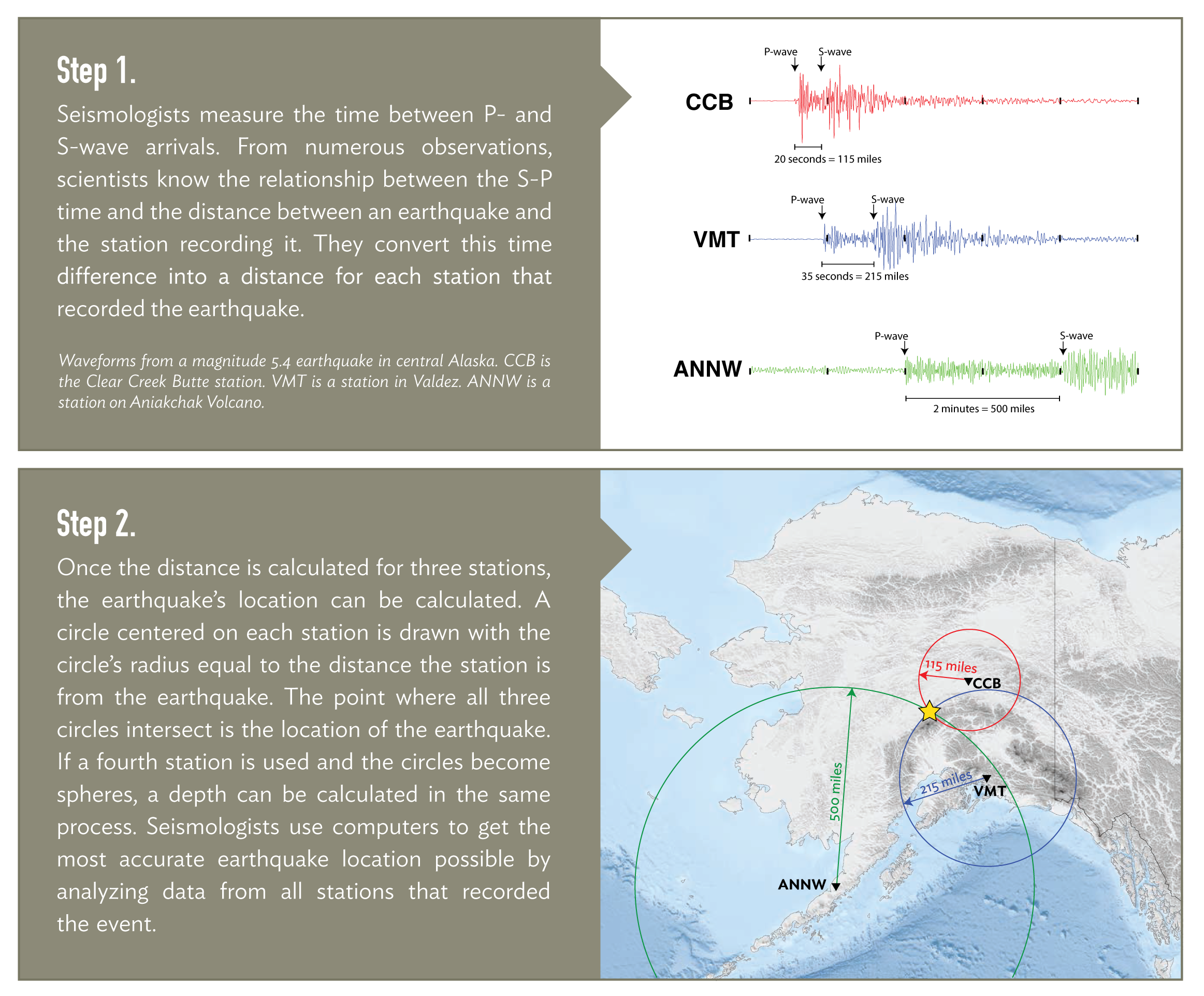
Different types of seismic waves move at different speeds. This means that if we know how much time passes between the arrival of faster P-waves and slower S-waves, we can calculate how far those waves traveled to the seismic station that recorded them. But this only tells us how far away an earthquake was, not where. To pinpoint the source on a map (the epicenter), we need to know how far it was from at least three points on the map. This means that if we have recordings of seismic waves arriving at three or more seismic stations, we can locate the earthquake using a method called triangulation (figure 1). A fourth station would be needed to determine the earthquake's depth.
This method is rudimentary, though, as it does not account for how the structure of the Earth affects seismic waves as they travel through it. The triangulation method assumes a constant velocity for each type of wave. In reality, seismic energy can bounce, bend, speed up or slow down as it passes through different materials. Properly accounting for those variations allows for a more accurate location. These “velocity models” are difficult to calculate and require a catalog of initial earthquake locations. Because of this, seismologists assume simple velocity models to get an initial earthquake location and then refine those locations depending on the level of detail needed.
Stage 1: Automatic locations
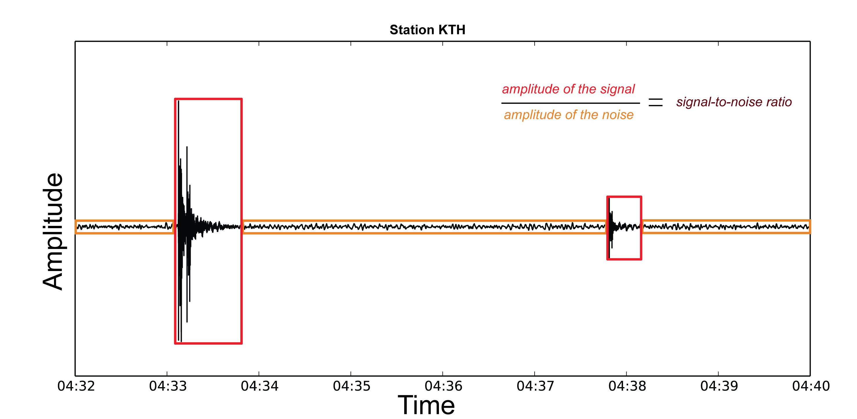
Because the Earthquake Center receives seismic data from hundreds of stations in real-time, we are able to use a computer program to generate initial locations. This program looks for characteristic peaks in the waveforms that occur across the network. It uses a signal-to-noise ratio (figure 2) to determine when a seismic signal (red) exceeds the background vibrations, also known as noise, (orange) constantly occurring in the earth.
When signals exceed a predetermined ratio on multiple stations, the program attempts to locate the presumed earthquake using a simplified model of the earth. The more arrivals and the better the distribution of stations, the more accurate the location will be.
Stage 2: Analyst reviewed locations
Analysts review each arrival and earthquake location that goes into our final earthquake catalog. The automated system misses some earthquakes and many arrivals, so analysts scan for these and add them manually. The automated system also tends to mark arrivals a little late or early, and in some cases it confuses non-seismic blips in the data with arrivals from earthquakes. Analysts refine or remove these accordingly.
Finally, depending on where the earthquake occurred, analysts must choose a velocity model. These models incorporate more of the complex structure of Alaska. Different models are used for the Aleutians, the southern mainland, and the northern mainland. The current velocity models produce accurate locations, but they do have a small degree of uncertainty associated with them.
Stage 3: High-precision relative earthquake locations
High-precision relative locations are often referred to as “relocations,” and in a sense they are relocated from their reviewed locations. A scientist doing a more thorough analysis of a region may want to reduce some of the uncertainty of reviewed earthquakes to better understand the fault on which the earthquakes occurred.
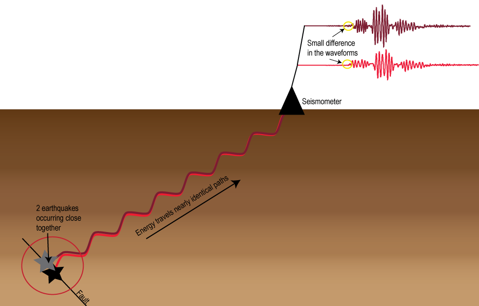
There are a couple of methods for computing high-precision relative locations, but they all rely on the same basic principles. If earthquakes occurring close enough together are recorded on the same station, then the seismic energy would have traveled the same path to get to the station (see figure 3). That means that any difference in their waveforms (yellow circles) can be directly related to their source area (red circle) because the path traveled would be the same. By comparing these differences, we can determine an earthquake’s location relative to all of the earthquakes around it instead of its distance from the recording station. This calculation results in a selection of earthquakes that are precisely located with respect to each other, so it gives a much clearer picture of the faults on which they occur.
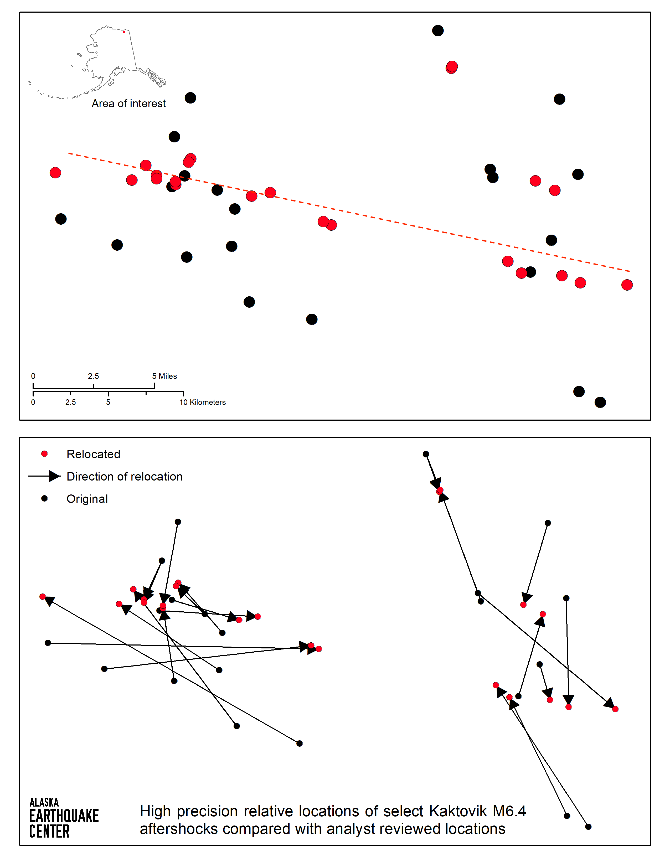
High-precision relative locations are most useful for aftershock sequences for large earthquakes. Aftershocks viewed on a map typically look like a cloud. High-resolution relocations can condense that cloud and better define the fault rupture of the mainshock. Figure 4 shows a selection of aftershocks from the M6.4 Kaktovik earthquake on August 12, 2018. The top panel shows the original locations (black) mapped with the relocations (red). Once relocated, the cloud of dots tightens up into an east-west trending line (red-dashed). The bottom panel connects the original location to the new location showing that some locations moved upward of 10 miles. The earthquakes are now located relative to each other as opposed to being individually located. Because the Kaktovik earthquake did not occur on a known fault, it was not immediately clear the orientation of the fault that ruptured. Initially, it was estimated that the M6.4 occurred on a north-south trending fault. However, this aftershock pattern suggests that the fault was most likely oriented east-west.