We use the phrase “magnitude of completeness” often when referring to our understanding of seismicity in a region or following a sequence of earthquakes. This value is a simplistic assessment of a catalog of earthquakes. By definition, the minimum magnitude above which we are reliably locating all earthquakes in a certain area is referred to as the magnitude of completeness (Mc). Sounds simple, right?
One complication is that this value is variable in time and space. Different regions of Alaska have a different Mc, and that value has changed through time. As seismic monitoring stations are added or removed, our ability to reliably locate small earthquakes changes. More closely spaced stations allow the Earthquake Center to locate smaller earthquakes and therefore lower the Mc. The loss of a station hinders our ability to locate smaller events, and raises the Mc.
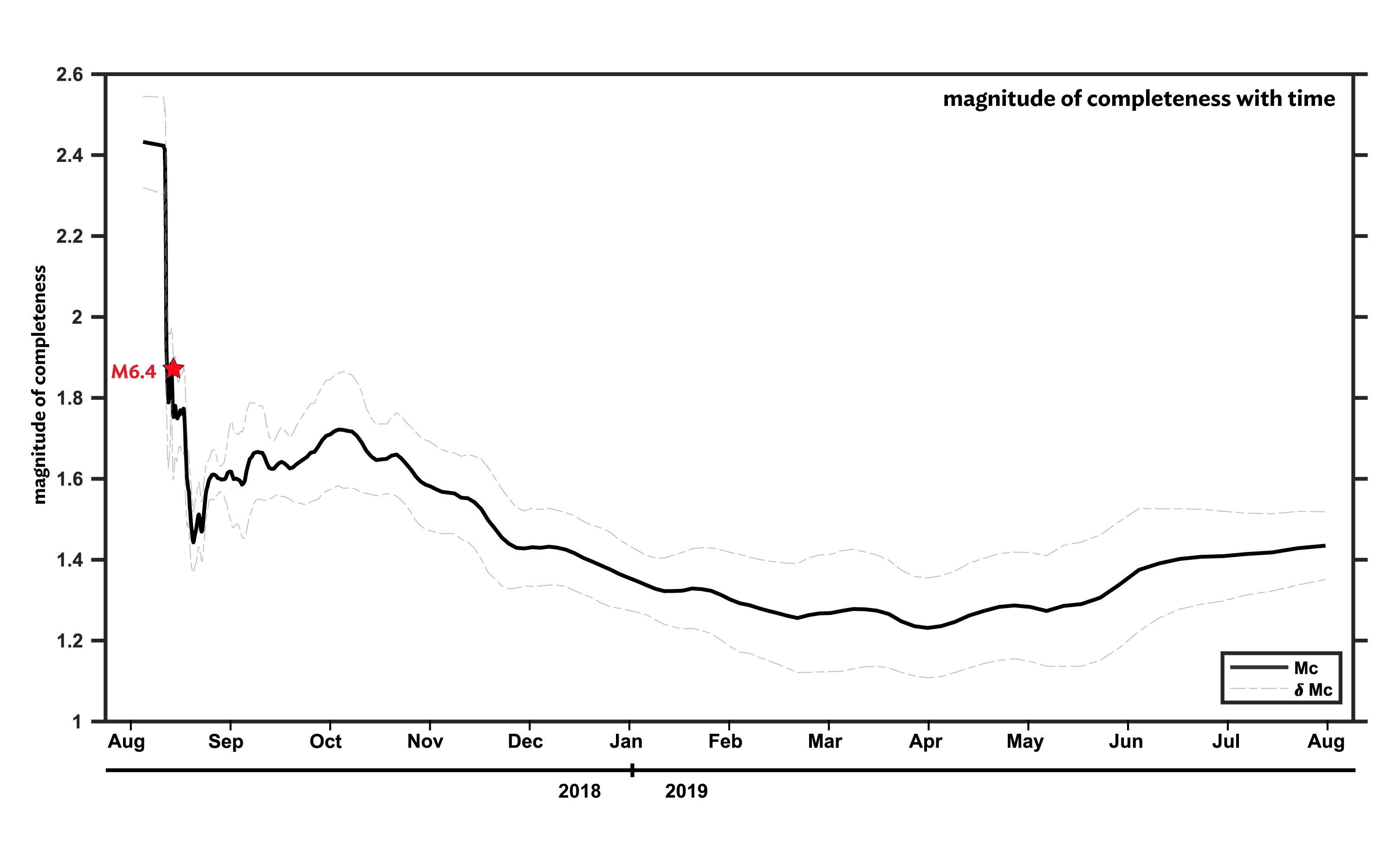
Another contributing factor is the rate of earthquakes. For example, early in an aftershock sequence there are often too many overlapping earthquakes. It becomes hard to separate multiple events and reliably locate small events. Over time, the sequence slows down and individual events are more easily seen (figure 1).
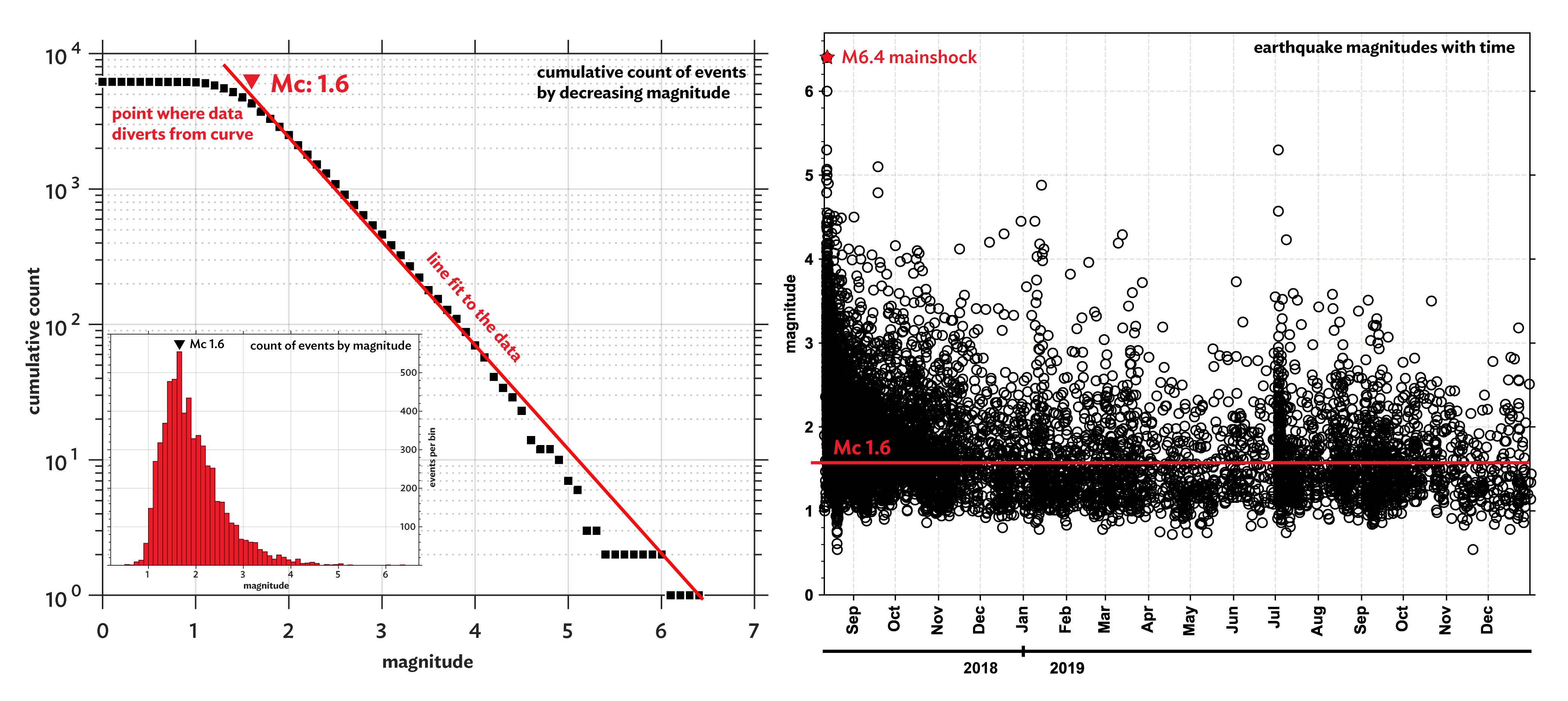
The most straightforward Mc estimation uses the Gutenberg-Richter Law of earthquake magnitude distribution developed in 1956. This method groups earthquakes into “bins” based on the number of events with magnitudes larger than each reference magnitude. For example, the M3 bin would include all events greater than or equal to 3 (figure 2, left inset). The count in each bin is then plotted on a common logarithmic scale. If this were a statistically perfect dataset, the data would form a straight line from M0 to M6.4. Statistically perfect datasets are nearly impossible, but we can use this relationship to estimate the Mc. When a straight line is fit to the data, the point where our data separates from the line is our magnitude of completeness.
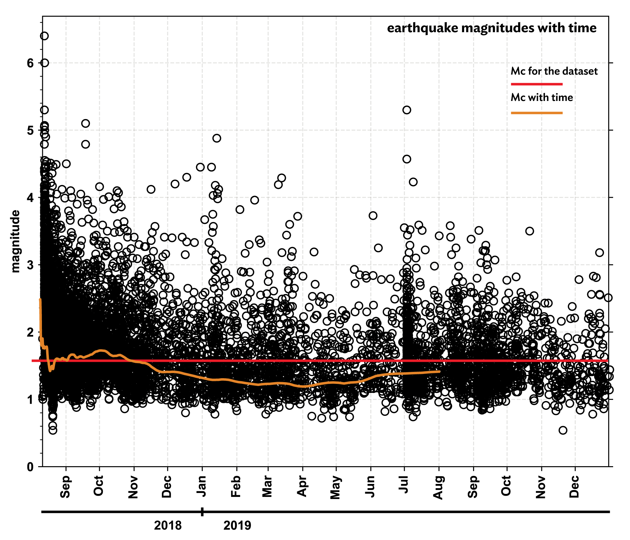
Why does this matter? Magnitude of completeness is a statistical way to determine the quality of an earthquake catalog. A strong regional (or sequence) catalog would have a low magnitude of completeness and would therefore better capture the whole seismic picture. Looking at the data in figure 2 (right), it would be tempting to assume a much lower Mc for the entire catalog. But as we see in figure 1, there are periods of time when the Mc is lower and times when it is higher. It’s important for seismologists to know the Mc of their catalog before beginning any analysis. For example, an incomplete catalog would result in unreliable or inaccurate findings, or, choosing a different time period may allow for the use of lower magnitude data (figure 3).
In the context of a regional network, such as the Alaska Earthquake Center, the Mc demonstrates where our monitoring capabilities are strongest and what areas might be lacking. While large-scale, damaging earthquakes show up across the network, background catalogs of smaller earthquakes in a region can help to determine the region’s seismic potential. The magnitude of completeness in the Aleutians is much higher than in Southcentral and Interior Alaska due in large part to sparser station coverage. It’s important to understand we may not be detecting as many small earthquakes there because of lack of equipment instead of lack of earthquakes. Measuring the Mc gives us a way to gauge how detailed our monitoring is in each region we cover.