Long gone are times when seismic arrivals were read off paper or film recordings by human eyes and manually processed with pen and paper. Nowadays, ground motion recordings from hundreds and thousands of miles away are available in our computer labs within seconds being transferred via internet, satellite or cell modem uplinks. The main challenge now lies in how to process these readily available gigabytes of data in the most efficient manner and provide the most accurate information quickly. As mentioned in the story on 3 stages of earthquake locations, we can use an automated system to generate an initial earthquake detection and location. 

The automatic detection procedure can be broken into two main stages: (1) detecting seismic arrivals - the more straight forward part and (2) using arrival information to identify earthquake locations and magnitudes - the more complicated part (for more information on magnitude see why magnitudes evolve in the minutes after an earthquake). 
 

Stage 1: Detecting seismic arrivals
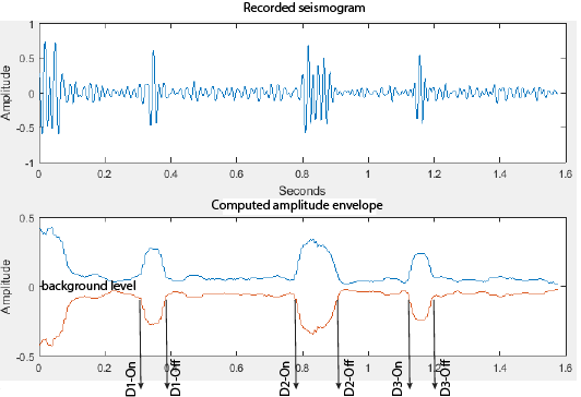
As the ground motion measurements make their way through the data acquisition system, a computer algorithm continuously scans each and every bit of data watching for seismic arrivals. The algorithm is trained to detect increases in ground motion amplitudes by comparing all incoming data to the recordings immediately preceding it, which we refer to as the background level. When the amplitude (signal) exceeds the background level (noise) by a certain, predefined factor and lasts a certain, predefined duration of time (known as a signal-to-noise ratio), a detection is declared by the algorithm and saved in a database (Figure 1). 

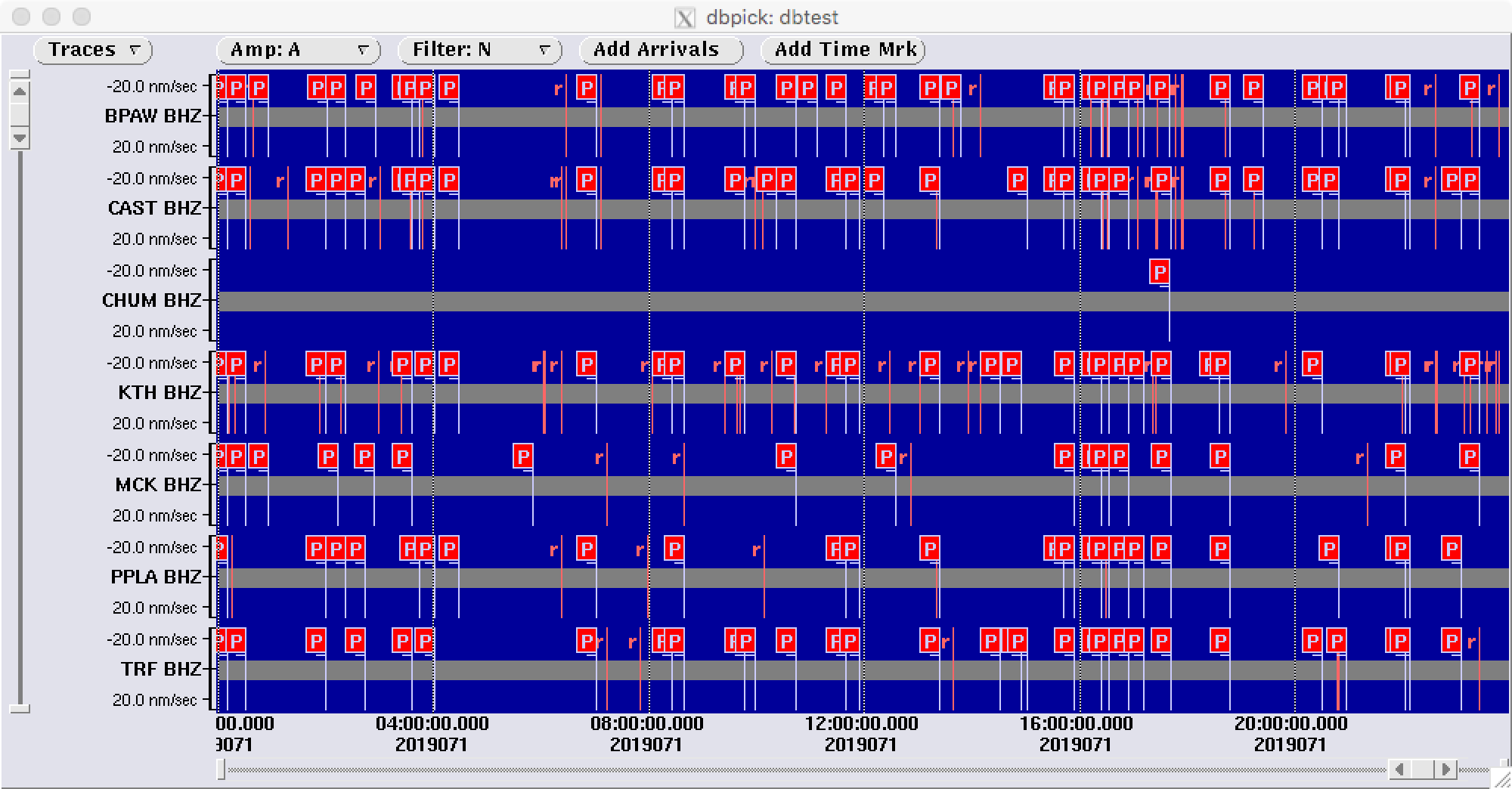
Routinely, hundreds of detections are being made in a span of a few hours, and even more when we deal with a particularly active aftershock sequence or an earthquake swarm. See the recent example of detections and arrivals from stations in and near the Denali State Park (Figure 2). 

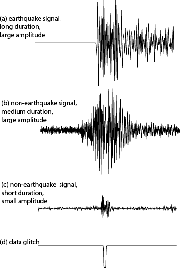
Our sensors are extremely sensitive and will record all kinds of ground motions, including an ice/rock fall on a nearby glacier, train or car passing by, heavy machinery working on a nearby construction project, and even animals passing over it. At first, the computer does not know if a given detection is an earthquake arrival or some other unrelated signal. To avoid creating too many false detections, we train the algorithm to only use signals of a certain strength and duration (see some examples in Figure 3). This way we can remove frequent and expected offenders: data glitches caused by field equipment malfunction; signals generated by different environmental factors such as wind busts, ice fractures, small rock falls, animal activities, etc. However, some non-earthquake signals are very good at mimicking the earthquake arrival behavior and make it into automatic detection lists. Therefore, the next step is to screen out some of these “rouge” detections based on timing and proximity to other stations with identified detections.

When an earthquake occurs, the seismic arrivals propagate in all directions at certain wave speeds. Since our goal is to detect seismic arrivals and to throw out all other un-related detections, we will only keep detections from seismic stations that are located within a certain distance of each other and that occurred within a given time window. For example, if a station is 100 miles away from an earthquake source, we expect the seismic arrival to show up there within about 15 seconds. If there are several stations, all within 100 miles from the earthquake source, we expect all seismic arrivals from this earthquake to occur within a 15 second time window. Since we know how large our state seismic network is, we can program time and distance limits into the algorithm. This way we can throw out a rouge detection from a site near Fairbanks when the rest of the detection list includes only sites on the Alaska Peninsula, located a thousand miles away. 
 

Stage 2: Associating arrival detections into earthquake locations
Once a list of screened “candidate” detections is obtained (we require at least five detections), another computer algorithm will attempt to compute the location and origin time of the event using the arrival times, recording station locations and a simplified model of the Earth.  

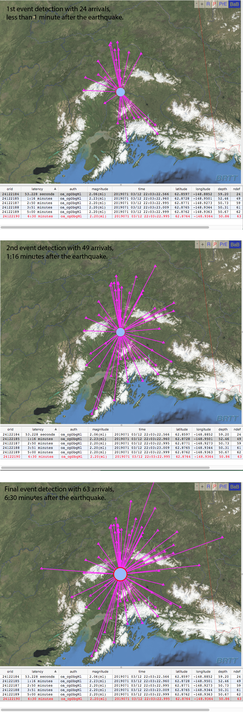
Because real-time data from field sensors continues rolling in, the detection list is constantly being updated with new arrivals. The location algorithm will keep updating the location as the detection list grows. (Figure 4). This will cause the location to adjust slightly in time and space. The more arrivals (detections) used and more distributed the station coverage, the better constrained the final location. With each location iteration, the magnitude is also calculated and updated.

Despite our best efforts to tune our automatic detection algorithms, bogus events may still be reported. For example, detections from two different earthquakes may be combined by the automatic system into a single event. This happens when earthquakes occur close in time and/or space. With so many different tectonic features generating earthquakes across the state, the likelihood of two or more earthquakes occurring at the same time is pretty high. Sometimes the system may have trouble separating two different earthquakes in a very active aftershock sequence, or our system will mistake an event that occurred in Japan or another distant region for something that occurred in Alaska.

We are thankful for modern computer technologies that allow us to sift through massive amounts of recorded ground motion data quickly and efficiently, but we still rely on our data analysts and seismologists to verify computer-generated earthquake detections. The human eyes remain the best tool to differentiate between real and bogus earthquake detections. This is changing, however, with rapid advancement of machine-learning and artificial intelligence in earth sciences. Stay tuned.